In Over  450 functions in Excel, MOD function is one of the highly overlooked. Generally, MOD function returns the remainder of two numbers after division.

Functions like IF, SUM, COUNT, AVERAGE are well known by all excel users. Yet there are some functions like MOD, WEEKDAY, WORKDAY, CHOOSE, DATEDIF, DELTA, SUBSTITUTE, HYPERLINK are rarely used.

This is part 1 of a series in which I endeavor to show you how these unpopular functions can be a lifesaver in many situations.

We shall start with MOD functions and after seeing how versatile it is you will wonder how come you have not used it so far.

Below are some of its uses;

1. Get a date of the most recent day of the week
2. Time & Date analysis
3. Highlight Whole numbers
4. Highlight every Nth Row
5. Sum Every Nth Value
6. Count Odd or Even Numbers
7. Fix Values every Nth Interval/Period

Basically, MOD function is used to get a remainder from a division

Syntax = MOD(Number, Divisor)

NB:

1. MOD always returns a result in the same sign as the divisor.
2. MOD will return a #DIV! error if the divisor is Zero

For example:

1. =MOD (7,5) result 2
2. =MOD(7,2) result in 1  because 2 goes into 7 thrice, with a remainder of 1

Get-Date of Most Recent Day of the Week

Excel stores date as sequential serial numbers so that they can be used in calculations. It also assigns a day of the week a number i.e. by default 1= Sunday to 7=Saturday.

Using these numeric values MOD can be able to fetch a date of a recent  day of the week given a start date and Number of the recent day

=StartDate-MOD(startDate-NumberOfRecentDay,7)

For example, to get a date of the recent Friday from Today, the formula would be

=Today()-MOD(Today()-6,7) 

Using the below example, Today (07-06-2016) is stored as number 42528,

MOD(Today()-6,7) =3 i.e  the recent Friday was 3 days ago

Therefore Friday’s date is (42528-3) since dates are stored as sequential serial numbers.

NB: If the “StartDate” weekday number is the same as the “NumberOfRecentDay”, “StartDate”  will be returned.

As you can see above since today (07-06-2016) is a Tuesday, then the recent Tuesday is returned as (07-06-2016).  To avoid this scenario use the below formula

=Today()-IF(MOD(Today()-6,7)=0,7,MOD(Today()-6,7))

Time & Date Analysis

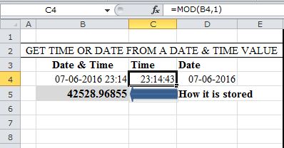
While Excel stores Dates as Serial Numbers, it stores time as a fractional portion of a 24 hr Day. For example, 8:00 Am is stored as (8/24)=0.33333333

MOD uses these numbers to;

• Extract Time from a DateTime Value

  =MOD(DateTime Value,1)

How it Works

When MOD is used with a divisor of 1, the result is the fractional part of the number, if any, because every whole number can be evenly divided by itself.

Convert Seconds into “Minutes:Seconds”

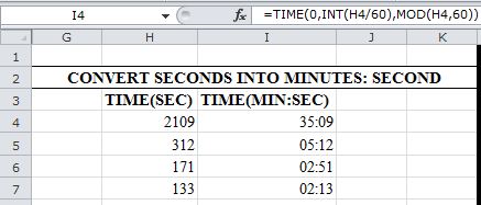
Using TIME and INT functions MOD can be used to convert Seconds into Minutes

  = TIME(0,INT(seconds/60),MOD(seconds,60)

How it Works

INT function ONLY returns the integer part of a decimal number. Therefore INT(2109/60) = 35

MOD(2109,60) returns the remainder from the divisor i.e 09

NB: This works ONLY when Time in seconds is NOT greater than one hour.

When the Time in seconds is greater than 1 hour, use the below formula: Remember to format your cell “h:mm:ss”

 =TIME(INT(seconds/3600), INT(MOD(seconds,3600)/60), MOD(MOD(seconds,3600),60))

For example to convert 8710 seconds into 2:25:10.

HOW?

INT(8710/3600) extracts the hours 2

INT(MOD(8710,3600)/60)→ INT(1510/60) → INT(25.1666666666667) extracts the minutes 25

MOD(MOD(8710,3600),60)→ MOD(1510,60) extracts seconds part 10

• Calculate Night Shift Hours

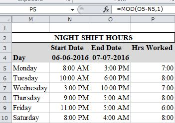
Calculating the time taken when the End-Time is Lesser than the Start-Time is tricky in excel.

For example calculating overnight hours results to negative values and Excel will display (#################)

To avoid these negative results, Use MOD which returns the  result in the same sign as the divisor

=MOD(EndTime-StartTime,1)

Highlight Whole Numbers

Since =MOD(Number,1) always results to Zero for whole numbers, we can use this in custom formatting to highlight Integers.

So =MOD(Number,1)=0 will always evaluate to TRUE on cells with Integers else FALSE. Condition formatting uses this Array of TRUE and FALSE to format the cells

How to go about it:

1. Go to Custom Formatting→Manage Rule→New Rule→Use a Formula to determine which cell to Format
2. Add the formula as shown below
3. Apply the format to the section required

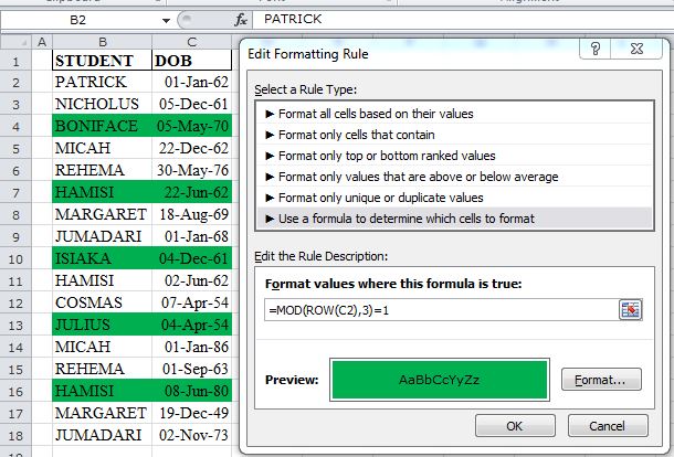
Highlight Every N^th Row

Use the same procedure outlined above but below function

= MOD(ROW(startCell),N)=1

For example, below formula highlights every Third row from the row that contains cell (C2) this is because it is the row that evaluates to TRUE

Sum Every N^th Value

With the combined powers of SUMPRODUCT and COLUMN Functions, MOD is able to Sum every Nth value in a Column.

= SUMPRODUCT(--(MOD(COLUMN(sumRange)-COLUMN(startColumn)+1,N)=0),sumRange)

How it Works:

• COLUMN(sumRange)-COLUMN(startColumn)+1→→ gets relative column numbers in a range ={1,2,3,4,5,6,7}
• (MOD({1,2,3,4,5,6,7},N)=0)→→Evaluates if the remainder is equal to Zero based on the divisor 

{FALSE,TRUE,FALSE,TRUE,FALSE,TRUE,FALSE}

• This  Boolean array is converted to Numbers equivalent by use of double negatives (double unary Method)

{0;1;0;1;0;1;0}

• SUMPRODUCT gets the sum of the product of the two arrays

=SUMPRODUCT({0;1;0;1;0;1;0},{260,270,190,370,630,120,620})

Count Even or Odd Numbers

MOD also combines with SUMPRODUCT in this calculation

         =SUMPRODUCT(--(MOD(countRange),2)=1)→→ For ODD numbers

        =SUMPRODUCT(--(MOD(countRange),2)=0)→→ For EVEN numbers

How it Works:

MOD returns a remainder of 1 for odd numbers and 0 for even numbers.

Fix Values Every N^th Period

Say you have a worksheet that manages overhead cost and you want to fix rent paid every third week, how can MOD function help?

=IF(MOD(COLUMN(startCell)-OffsetValue,N)=0,FixValue,0)

NB: OffsetValue is determined by the number of columns your startCell column is from column A

Another method as suggested in the comments below is

=(MOD(COLUMN(StartCell)-offsetValue ,N)=0)*FixValue

MOD FUNCTION EXAMPLES WORKSHEET

Conclusion:

I hope I have made a point that MOD is not a Function to ignore anymore. If you have not been using it–Start today.

I am also sure the list above is not exhaustive, so Leave a Comment and add more way to use MOD FUNCTION

Recommended Link:

https://www.automateexcel.com/most-useful-excel-functions

https://excelsemipro.com/2010/08/convert-seconds-to-a-time-format-in-excel/