

Extracting numbers from a string in excel is a must-have skill in data cleaning.
There are different methods of this extraction depending on the position of the numbers.
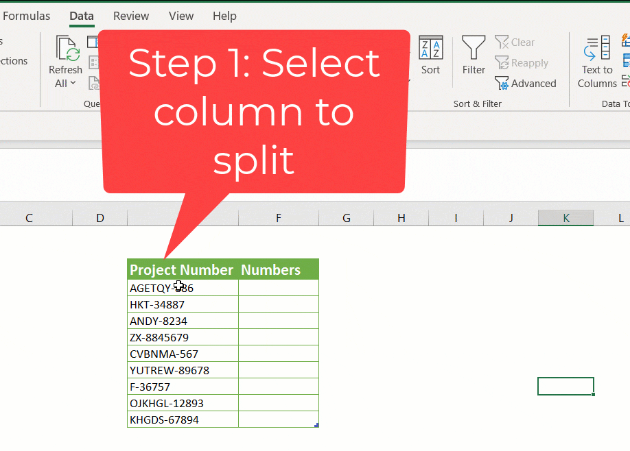
Extracting numbers at the end of a string
Scenario 1: There is a separator between text and numbers

Use Text to Columns
Use the Flash fill tool
This is the simplest as all you have to do is to give excel an example and then press Ctrl + E

NB: As simple as this method may be, be careful to check the final results as it does not always give correct results.
Use a formula
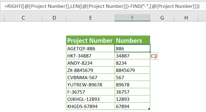
How the formula works:
⭐ FIND(“-“,[@[Project Number]]) returns the position of the separator in the string
⭐ LEN([@[Project Number]]) returns the length of the string
⭐ LEN([@[Project Number]])-FIND(“-“,[@[Project Number]]) returns the number of characters after the separator
⭐ RIGHT([@[Project Number]],LEN([@[Project Number]])-FIND(“-“,[@[Project Number]])) extracts the above number of characters from the right of the string
NB: This is the only dynamic method–unlike the above 2 methods if the string changes the method is able to extract the numbers.
PS: Text to Columns & Flash fill will also work if numbers are at the beginning of the string
The formula changes in the case of extracting numbers at the beginning of a string
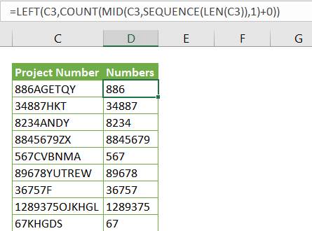
How the formula works,
MID(C3,SEQUENCE(LEN(C3)),1) splits the string into separate characters {“8″;”8″;”6″;”A”;”G”;”E”;”T”;”Q”;”Y”}
Since you want to count the numbers in the string, add zero to convert to the number MID(C3,SEQUENCE(LEN(C3)),1)+0 this results in {8;8;6;#VALUE!;#VALUE!;#VALUE!;#VALUE!;#VALUE!;#VALUE!}
COUNT function ignores the #VALUE! error and returns just numbers count
The LEFT function extracts the characters from the left of a string based on the count number.
Scenario 2: There is NO separator between text and numbers
Unlike the above scenario, you cannot use the Text to Column method there.
You may use the flash fill method but be very careful as it does not always give the correct results
Use a Nested function
How the Formula Works
SEQUENCE(10,,0) returns an array of all possible numbers {0,1,2,3,4,5,6,7,8,9}
- If you don’t have Office365 you can replace it with this array
SEARCH(SEQUENCE(10,,0),C3&SEQUENCE(10,,0)) returns the position of any of the numbers in the text
MIN(SEARCH(SEQUENCE(10,,0),C3&SEQUENCE(10,,0))) returns the 1st position that a number occurs in the text
To include this first number in the extraction, add 1 (MIN(SEARCH(SEQUENCE(10,,0),C3&SEQUENCE(10,,0))))+1
LEN(C3)-(MIN(SEARCH(SEQUENCE(10,,0),C3&SEQUENCE(10,,0))))+1 returns a count of the number characters
RIGHT function extracts these number characters
NB: If you do not have Office365 use below formula
=RIGHT(C3,LEN(C3)-(MIN(SEARCH({0,1,2,3,4,5,6,7,8,9},C3&{0,1,2,3,4,5,6,7,8,9})))+1)
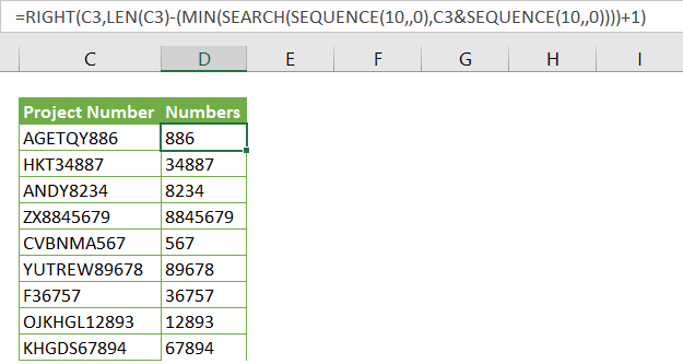
Extracting numbers mixed in a string
IFERROR(MID(B3,SEQUENCE(LEN(B3)),1)+0,””))
Incase you don’t have Office365 you can replace the SEQUENCE function with ROW(INDIRECT(“1:”&LEN(B3)))
=TEXTJOIN(“”,TRUE,
IFERROR(MID(B3,ROW(INDIRECT(“1:”&LEN(B3))),1)+0,””))
If you do not have the TEXTJOIN function, you can use the CONCAT function as shown below
=CONCAT(
IFERROR(MID(B3,ROW(INDIRECT(“1:”&LEN(B3))),1)+0,””))
If you are using Office 2013 and below try below formula…thanks to Muhammad Nauman
=SUM(MID(0&B3, LARGE(INDEX(ISNUMBER(0+MID(B3,INDEX(ROW(INDIRECT(“1:”&LEN(B3))),,),1))*(INDEX( ROW(INDIRECT(“1:”&LEN(B3))),,)),0), INDEX(ROW(INDIRECT(“1:”&LEN(B3))),,))+1,1) * 10^(INDEX(ROW(INDIRECT(“1:”&LEN(B3))),,))/10)
Find and Replace ALL LETTERS in Excel
To replace all letters once follow the steps below:
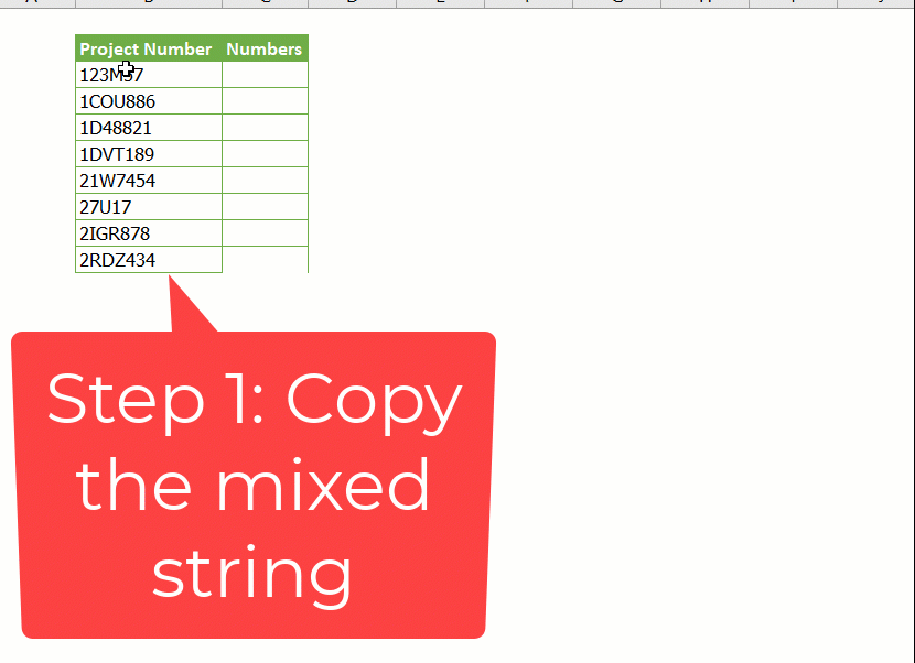
- Copy all the mixed string
- Open a new Microsoft Word Document
- Paste the data there
- Click Ctrl + H
- Go to Special and Select Any Letter
Using Power Query to Extract Numbers from a String
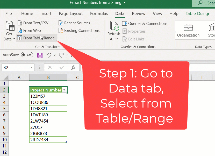
Text.Select([Project Number],{“0”..”9″})
Learn more about Power Query Text Functions

You cited a formula by Muhammad Nauman in the section for extracting digits in a mixed string for those using XL2013 and earlier. I believe this shorter formula will also work…
=MID(SUMPRODUCT(–MID(“01″&A1,SMALL((ROW($1:$300)-1)*ISNUMBER(-MID(“01″&A1,ROW($1:$300),1)),ROW($1:$300))+1,1),10^(300-ROW($1:$300))),2,300)
**Commit formula using CTRL+SHIFT+ENTER
Note that, as written, cell A1 cannot contain more than 300 characters total and that the formula can only return a maximum of 14 total digits.
how to extract specific number from a string of numbers in row, eg
0 0 0 0 8 0 0 2 3 0 0 – how to extract number 8?
Assuming your string is in cell G15
=INDEX(MID(G15,SEQUENCE(LEN(G15)),1),
MATCH(TRUE,ISNUMBER(FIND(“8”,MID(G15,SEQUENCE(LEN(G15)),1))),0))
Tried “=RIGHT(C3,LEN(C3)-(MIN(SEARCH(SEQUENCE(10,,0),C3&SEQUENCE(10,,0))))+1)” but it always returned the entire cell’s text. Worked only when the cell contained ONLY a number formatted as text, e.g. “90.25%”. Confirmed I am using Excel 365. Not going to try the array version because I have several thousand rows.
Please provide a sample workbook so that I can see where the problem is
how to take account number out of cell
123 Louisville Gas
4567 Louisville Water Company
89 Spectrum
1 Waste Management
I want the number in one cell and the company in another.
Hi Kim,
Try below formula
=CONCAT(IFERROR(MID(A1,SEQUENCE(LEN(A1)),1)+0,””))
Assuming your text is in cell A1
Hi, How to take Total of this formula (right side of the ‘&’ only) to another cell.
=”SFD869: “& 100000-22500-1900-2500-500
Use this function
=SUM(IFERROR(TEXTSPLIT(TextString,,{“&”,”-“})+0,””))
how to get only the serial number on the following example http://go2se.com/ref=WXXXX–/sn=085476328804
If you have office365 use below function
=TEXTAFTER(B2,”sn=”)
What could you use with these formulas to where it extracts number after strings that might also contain a number.
For example, using your methods I can get 9513 from SUP:SUB9513.
However, I need to get 10849 from SUP:L-310849.
This is using Excel 2019. We haven’t switched to 365 yet.
Hi Page,
Are they always the last 5 numbers?
If Yes, then use the right function =RIGHT(B2,5)+0
If not tell me what pattern they follow
How do I separate these into two columns – column 1 has 1, 2, 3,… column 2 has 5537.25, 5189.07, 7287.69,….
Name: LOTS : 1
Area: 5537.25 Sq. Ft.
Name: LOTS : 2
Area: 5189.07 Sq. Ft.
Name: LOTS : 3
Area: 7287.69 Sq. Ft.
You can use the TEXTSPLIT or FILTERXML functions.
Send me a workbook sample
I have this formula : =(ASAPEXTRACTNUMBERS(CONCATENATE(O13))), which returning back a string with all numbers in a cell, but I need the minimum value instead of a serie of number. eg. original cell contains:
Functional Test.: 4
In- Circuit Test: 4
Inspection, Visual: 7
Run-in Test: 4
Use below DAF
=MAX(IFERROR(TEXTAFTER(TEXTSPLIT(C3,CHAR(10)),”:”)+0,””))
If you do not have Office365, use below function
=MAX(ISNUMBER(FIND(ROW($1:$100),C3))*ROW($1:$100))
Hello, I am looking to find a formula to calculate the number of visits someone has remaining on a package, however the string shows the number of visits used. The string is “Physical Therapy Initial Evaluation – 1/1 Physical Therapy Follow-Up Visit – 3/9”. I would like it to show as “6” as the person has used 3 out of 9 visits and has 6 remaining. Thanks for your help!
Please send a sample worksheet…Textsplit can work
Hi! for the Extracting numbers mixed in a string option, it was not working for me until I wrote “Arrayformula” before the MID function. Hope it helps someone else!
Thanks for the info
There’s also a long way by using the substitute formula assuming you’re looking at cell A1.
For removing Numbers:
=SUBSTITUTE(SUBSTITUTE(SUBSTITUTE(SUBSTITUTE(SUBSTITUTE(SUBSTITUTE(A1, “0”, “”), “1”, “”), “2”, “”), “3”, “”), “4”, “”), “5”, “”), “6”, “”), “7”, “”), “8”, “”), “9”, “”)
For removing letters:
=SUBSTITUTE(SUBSTITUTE(SUBSTITUTE(SUBSTITUTE(SUBSTITUTE(SUBSTITUTE(SUBSTITUTE(SUBSTITUTE(SUBSTITUTE(SUBSTITUTE(SUBSTITUTE(SUBSTITUTE(SUBSTITUTE(SUBSTITUTE(SUBSTITUTE(SUBSTITUTE(SUBSTITUTE(SUBSTITUTE(SUBSTITUTE(SUBSTITUTE(SUBSTITUTE(SUBSTITUTE(SUBSTITUTE(SUBSTITUTE(SUBSTITUTE(SUBSTITUTE(A1, “A”, “”), “B”, “”), “C”, “”), “D”, “”), “E”, “”), “F”, “”), “G”, “”), “H”, “”), “I”, “”), “J”, “”), “K”, “”), “L”, “”), “M”, “”), “N”, “”), “O”, “”), “P”, “”), “Q”, “”), “R”, “”), “S”, “”), “T”, “”), “U”, “”), “V”, “”), “W”, “”), “X”, “”), “Y”, “”), “Z”, “”)
Awesome Alternative!!!
need to extract data between multiple cells containing text & numbers Example:
if cell A1 texts like CAI I need the result to be SLB // IF CONTAIN NUMBER like 222 I need the results to be VIVO ALEX
Plz note: maybe the same cell contains a mix between (Numbers & Texets )
Colum A ColumB
CAI SLB
EBE SLB
BAG SLB-Bag
SCCR SLB
222 VivO ALX
ENO WAS
223 VivO CAI
I want to extract 9 digit numerical value out of a text,
Sample : S.No. 747780507, Key No. RG5TK734R
suggest.
If you have office365 use below function
=CONCAT(TOCOL(MID(H9,SEQUENCE(LEN(H9)),1)+0,2))
Watch this video for more:
https://www.youtube.com/watch?v=-AGzgxjuUcU