How to Return Multiple Columns in VLOOKUP Function

By default, VLOOKUP is set to return a Single column but with a small tweak, it can return multiple columns.

=VLOOKUP(G2,B2:E24,{3,4},FALSE)

The only trick is to put the multiple columns in curly braces.

NB:

You can insert the column numbers in any order.

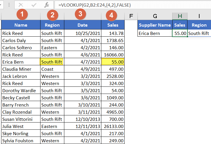
For example, if you want to return the Sales (column 2) and Region (Column 4) in that order then use the below formula

=VLOOKUP(G2,B2:E24,{4,2},FALSE)

DOWNLOAD WORKSHEET

How to Use Multiple Criteria in a VLOOKUP function

VLOOKUP IS DEAD–OR IS IT?