Have you ever looked for an Excel function that is extremely powerful, flexible and has multiple uses? The ONE function that will solve most of your daily array of problems? The ONE function that will open doors to advanced Excel skills?

Well! This is it—SUMPRODUCT.

SUMPRODUCT can be used to:

1. One way lookup  with multiple condition(s)
2. Conditional sum
3. 2-way lookup
4. 2-way lookup with multiple conditions(s)
5. Sum top or bottom N items
6. Text analysis
7. Conditional summaries
8. Count unique values in a range
9. Counting fields with Errors or blank or text or numbers
10. Check if a number is ODD or EVEN plus count the same in a range
11. Count the number of times a list of values occur in a range
12. Monthly/Yearly Analysis

So what is SUMPRODUCT Function?

Basically, SUMPRODUCT calculates the sum-of-the-product of matching numbers in given arrays i.e from 2  to a maximum of 30 arrays.

Some rules:

1. All Arrays should be of equal size otherwise, SUMPRODUCT returns the #VALUE! error value.
2. Arrays cannot be a mix of columns and rows.

   = SUMPRODUCT(Array1,Array2,…………,Array30)

For Example, to calculate total sales from below example, you need to sum the product of Sold Qty*Sales Price*Shipping Cost

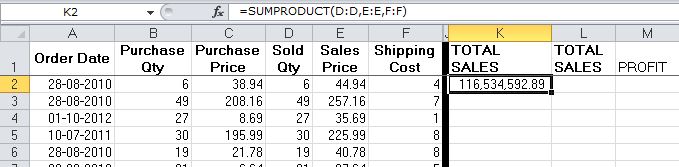
Lookup, Get-Product, and Sum-the-Product All at one

You can incorporate condition(s) in SUMPRODUCT to perform conditional sum or count.

For example to generate a summary of sales per product category you can use SUMPRODUCT with criteria as shown below;

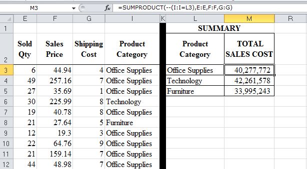
=SUMPRODUCT(--(Critera range=Criteria), Array1, Array2, Array3)

NB:

• --(Critera range=Criteria) the  two dashes are added (Double unary) are used to convert an internal array of TRUE/FALSE into 1/0

How It works:

• (Category range=”Furniture”) will evaluate to True in all the cells whose category is Furniture and False in all other cells

 {TRUE;TRUE;TRUE;FALSE;TRUE;FALSE;TRUE;TRUE...}

• To convert this Boolean array to its Numbers Equivalent we use the double negatives (double unary Method)

{1;1;1;0;1;0;1;1...}

• SUMPRODUCT then uses 1/0 array to multiply with the Sales qty, price & shipping cost

NB:

• You can add more conditions (criteria) on sumproduct to get drilled down summaries.

 Use * where conditions MUST be met for the argument to be evaluated TRUE

For example, breakdown the sales cost of Furniture  for the year 2009 only;

=SUMPRODUCT((Product category=”Furniture”)*(Year=2009), Qty,Price,Shipping Cost)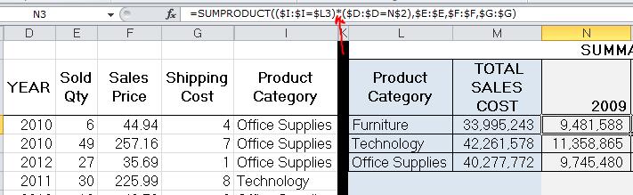

Use +  where EITHER condition is met for the argument to be evaluated TRUE

For example to calculate the sales for Furniture or Technology in the year 2010 then:

=SUMPRODUCT(((Category=”furniture”)+(Category=”Technology”))*(Year=2010), qty,Price, shipping)

2 WAY LOOKUP

To Lookup is to use a value in one column/row and find and get a corresponding value from another column/row(s).

As for a  2 Way Lookup, you find and get a value at the intersection corresponding to a given row(s) & column(s) values.

For example, you can calculate how many quantities were Ordered by KIM on 28-08-2010 using below data.

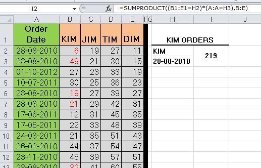
=SUMPRODUCT(dates=”28-08-2010”)*(customers=”KIM”)*(ordersData))

NB: You have to select the whole ordersData (highlighted in Gray) not just the column for KIM orders.

Counting fields with Errors, odd/even numbers, blank, text, Non-text e.t.c

 =SUMPRODUCT(--ISERROR(array)) 

How it works:

• --ISERROR(array) will evaluate to True in all the cells containing errors and False in all other cells. We use the double unary method to convert an internal array of TRUE/FALSE into 1/0
• SUMPRODUCT then adds up the 1/0 array

SUMPRODUCT({1,0,0,1,1,0..})

NB: 

You can replace ISERROR with ISBLANK, ISTEXT, ISNUMBER, ISNONTEXT but not with “ISEVEN” or “ISODD”

Counting ODD or EVEN numbers use MOD function

=SUMPRODUCT(--(MOD(array,2)=1)) counts field with odd numbers

NB:

MOD returns a remainder of 1 for odd numbers and 0 for even numbers.

How it works:

• --(MOD(array,2)=1) will evaluate to True in all the cells containing odd numbers and False in all other cells. We use the double unary method to convert an internal array of TRUE/FALSE into 1/0
• SUMPRODUCT then adds up the 1/0 array

SUMPRODUCT({1,0,0,1,1,0..})

Counting Text Field Based on the Number of their Characters

  =SUMPRODUCT(--(LEN(array)=n)) 

For example to count text field whose length is 4 characters then

  =SUMPRODUCT(--(LEN(array)=4)) 

How it works:

• --(LEN(array)=4) will evaluate to True in all the cells containing text whose length is 4 characters and False in all other cells. We use the double unary method to convert an internal array of TRUE/FALSE into 1/0
• SUMPRODUCT then adds up the 1/0 array

SUMPRODUCT({1,0,0,1,1,0..}).

Counting Unique Values in a Range

=SUMPRODUCT(--(FREQUENCY(range,range)>0))  

Formula excludes Blank cells

See Explanation here

Counting  Values Repeated N times

=SUMPRODUCT(--(FREQUENCY(range,range)=N))  

formula excludes Blank cells too

See Explanation here

Calculating Weighted Average

=SUMPRODUCT(array1,array2)/sum(array2)   

NB: Array2 being the weights

Sum the Top N Values in a Range Without Duplicates

 =SUMPRODUCT(LARGE(SumRange,ROW(INDIRECT("1:N")))) 

How it Works

For example, calculate the top 3 sales using below data

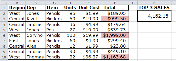
=SUMPRODUCT(LARGE(F2:F10,ROW(INDIRECT("1:3")))) = 4,162.18

►ROW(INDIRECT(“1:3”) evaluates to {1;2;3} which forms the k part of LARGE function

►LARGE(F2:F10,{1;2;3}) fetches the top 3 values {1999;1163.68;999.5}

►SUMPRODUCT({1999;1163.68;999.5}) adds up the items in the array

                              Or Use below formula

=SUMPRODUCT(SumRange,--(RANK(SumRange,SumRange)<=N))

How it Works

For example, calculate the top 3 sales using below data

=SUMPRODUCT(F2:F10,--(RANK(F2:F10,F2:F10)<=3))=4,162.18

►RANK(F2:F10,F2:F10) assigns a ranking number for all the items in the range {7;3;8;4;1;6;9;5;2}

►–(RANK({7;3;8;4;1;6;9;5;2})<=3) will evaluate to True in all the cells whose rank is greater or equal to 3 and False in all other cells. We use the double unary method to convert an internal array of TRUE/FALSE into 1/0  i.e .  {0;1;0;0;1;0;0;0;1}

►=SUMPRODUCT(F2:F10,{0;1;0;0;1;0;0;0;1}) SUMPRODUCT multplies the two arrays and adds up their products.

NB:

To sum the Bottom N Values, Rank the range Ascending

=SUMPRODUCT(SumRange,--(RANK(SumRange,SumRange,1)<=N))

Counting Items Based on Two or More Criteria

For example how many times did we sell furniture in the year 2010?

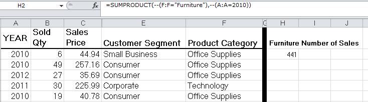
=SUMPRODUCT(--(F:F="Furniture"),--(A:A=2010))

Find the Last Occurrence of Item in List

When combined with INDEX, SUMPRODUCT can be used to fetch the last occurrence of items in a list—The List  should be arranged descendingly

For example, fetch the last time Home Office ordered?

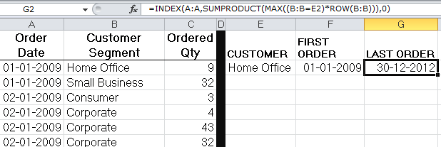
=INDEX(orderdate,SUMPRODUCT(MAX((customer="Home Office")*ROW(customer))),0)

Conclusion:

If INDIRECT is Excel’s Most Evil Function because of its Volatility, then SUMPRODUCT is Excel’s Most Powerful Function because of its Versatility.

Download SumProduct Worksheet

Learn More On SUMPRODUCT from below links:

2 WAY LOOKUP IN EXCEL

SUMPRODUCT WITH WILD CARDS

https://exceluser.com/formulas/last-item-in-list.htm

https://www.excelhero.com/blog/2010/01/the-venerable-sumproduct.html

https://www.xldynamic.com/source/xld.sumproduct.html#top

https://www.meadinkent.co.uk/xlsumproduct.htm