When is the last time you used the REPT function in Excel?
REPT is one of excel’s little-known, overlooked, and underutilized function, yet very useful.
Generally, REPT returns a specific text string a specified number of times.
=REPT(“Text”, Number of times)
Here are 7 ways you can start using REPT function.
- ADD LEADING ZEROS
- CREATE INLINE CHARTS
- REPLACE NESTED IF
- CREATE A MIRROR GRAPH
- CREATE-STEM AND LEAF PLOTS
- EXTRACT N WORDS FROM A TEXT STRING
- CREATE A STAR RATING SYSTEM
ADD LEADING ZEROS
By default, Excel removes any leading zero in a number yet there are instances where these are required.
For example, suppose you want to convert numbers to cost codes? or store phone numbers?
Note, the cost codes should start with a zero and must have 10 characters
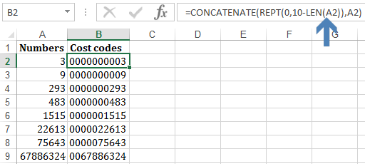
=CONCATENATE(REPT(0,10-LEN(A2)),A2)
How it works:
►10-LEN(A2)–Calculates the number of times to repeat Zero.
Since we need 10 characters in the cell, then the number of times the leading zeros are repeated should be 10 minus the length of the number.
CONCATENATE function just joins the repeated zeros with the number. You can also use an ampersand to join the two
=REPT(0,10-LEN(A9))&A9
CREATE INLINE CHARTS
Inline charts are very important in creating dashboards. With simple REPT function, you can build a dynamic inline chart as shown below

=REPT(“|”,B2*10)
How it works
► After inserting the formula on row 3, change the font to Playbill, make it bold with size 28
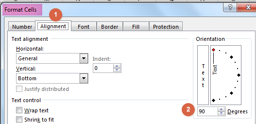
►Realign the contents in row 3 to 90°. Go to cell format, alignment, set to 90 degrees
►Apply conditional formatting to the charts based on the costing percentages. Go to conditional formatting, manage rules then new rule, then set your rules.

REPLACE NESTED IF
As shown in this article, 7 alternatives to Nested IF, you can speed your spreadsheet calculations by replacing nested IF functions with REPT
For example, suppose you have below production figures and you want to return it the status
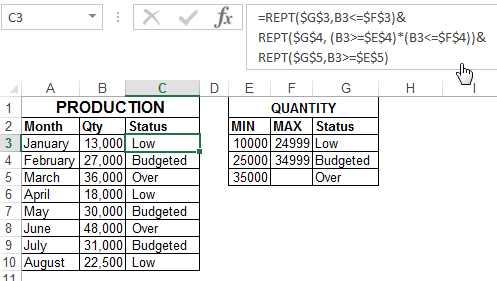
=REPT($G$3,B3<=$F$3)&
REPT($G$4, (B3>=$E$4)*(B3<=$F$4))&
REPT($G$5,B3>=$E$5)
How it works
Internally, Excel recognizes the value of TRUE as 1 and the value of FALSE as 0. Also, REPT functions return an empty string if the number to return is zero. These are the fact that REPT utilizes in the above function.
Firstly, REPT function evaluates every condition and returns a TRUE or FALSE.
Since ONLY 1 condition will evaluate TRUE, REPT function returns a string of empty strings and one status value.
="Low"&""&""
CREATE A MIRROR GRAPH
Mirror graphs are among the hardest to create in my opinion yet among the best in comparing 2 sets of data.
I had been struggling to find an easy and flexible way until I found REPT function.
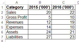
For example, how do you transform above data to below mirror chart?
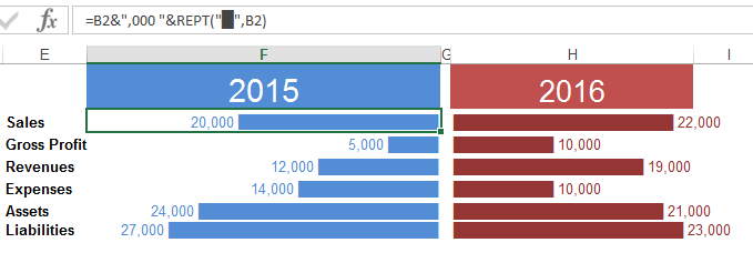
Steps:
► Insert REPT function in Column F. On the text to repeat type “Alt+220” this will repeat this character ▄
►On the numbers to repeat, reference the units per category and join them with “,000” text string.
► For the data in column F, ensure you align your content to the right.
►Change the text font appropriately.
CREATE STEM & LEAF PLOTS
A Stem and Leaf Plot is a special table where each data value is split into a “stem” (the first digit or digits) and a “leaf” (usually the last digit). More like a frequency distribution table.
For example, how do you create a stem & leaf plot for below quantity data?
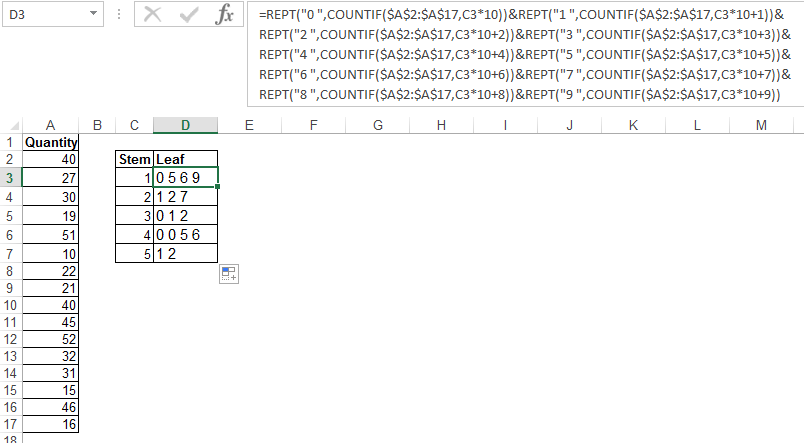
=REPT("0 ",COUNTIF($A$2:$A$17,C3*10))&
REPT("1 ",COUNTIF($A$2:$A$17,C3*10+1))&
REPT("2 ",COUNTIF($A$2:$A$17,C3*10+2))&
REPT("3 ",COUNTIF($A$2:$A$17,C3*10+3))&
REPT("4 ",COUNTIF($A$2:$A$17,C3*10+4))&
REPT("5 ",COUNTIF($A$2:$A$17,C3*10+5))&
REPT("6 ",COUNTIF($A$2:$A$17,C3*10+6))&
REPT("7 ",COUNTIF($A$2:$A$17,C3*10+7))&
REPT("8 ",COUNTIF($A$2:$A$17,C3*10+8))&
REPT("9 ",COUNTIF($A$2:$A$17,C3*10+9))
How it works:
The formula is scary big but fairly easy to understand once you break it down:
►COUNTIF($A$2:$A$17,C3*10)–counts how many tens, the twenties, thirties e.t.c occur in the range.
►REPT(“0 “,COUNTIF($A$2:$A$17,C3*10))–returns Zero the number of times these tens, twenties e.t.c occur
►COUNTIF($A$2:$A$17,C3*10+1)–to cater for the occurrences of ones of these tens, the twenties e.t.c, we add either 1, 2 , 3, 4, 5, 9, 7, 8, 9 in our COUNTIF function
►REPT(“1 “,COUNTIF($A$2:$A$17,C3*10+1))–for example, this part of the formula returns 1 the number of times 11 occurs
NB: If you need more explanation Watch this Video
EXTRACT n WORDS FROM A TEXT STRING
It is easy to extract characters from a string if you know the number of characters to extract.
MID, RIGHT, and LEFT functions are mostly used in these string manipulation.
But, how do you extract the last 3 words from the below sentences? how do you find the 3rd single space, from the right, and extract all words after it?

=TRIM(RIGHT(SUBSTITUTE(A2," ",REPT(" ",LEN(A2))),3*LEN(A2)))
How it Works
Since the last 3 words are of different lengths from sentence to sentence, we need to find a way to use the 3rd last single space as our criteria to extract them.
REPT(” “, LEN(A2))–takes all single spaces in the sentence repeats them a number of times equal to the length of the sentence.
SUBSTITUTE(A2,” “, REPT(” “, LEN(A2)))–finds the single spaces and replaces them with the repeated spaces from REPT function.
Since you now know the relative position of the spaces, you can use RIGHT function and the LEN function to find the last 3 words
RIGHT(SUBSTITUTE(A2,” “,REPT(” “,LEN(A2))),3*LEN(A2))

Since the words extracted by RIGHT function still has the repeated spaces, use the TRIM function to cut all extra spaces except single spaces between words.
NB: For more explanations, WATCH THIS VIDEO
CREATE A STAR RATING TEMPLATE
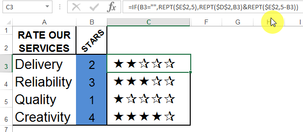
=IF(B3="",REPT($E$2,5),REPT($D$2,B3)&REPT($E$2,5-B3))
How it works:
Go to Insert ►Symbols ► Select Wingdings under font ►Insert two starts (☆★) on separate cells

IF(B3=””,REPT($E$2,5)–in case the ratings are blank,repeats the blank star 5 times
REPT($D$2, B3)&REPT($E$2,5-B3)–in the case of a rating, repeat the full star the number of rating score and the blank star 5 minus the rating score.
Edit: 2nd July:
After posting the article on Linkedin, Abhijeet R. Joshi suggested a tweak simplifying the star rating.

Instead of inserting the symbols first, referencing them and repeating them, you can just hard-code them in the function.
=IF(B3="",REPT(CHAR(182),5),REPT(CHAR(171),B3)&REPT(CHAR(182),5-B3))
Ensure you change the font in column C to Wingdings.
NB: Check out an alternative of creating these star rating
DOWNLOAD REPT function WORKSHEET
Related Links
7 OVERLOOKED USES OF EXCEL MOD FUNCTION
EXCEL’S WEEKDAY FUNCTION IN-DEPTH
SUMPRODUCT–EXCEL’S MOST POWERFUL FUNCTION
Inspiration Sites for the Article:
Read more on Stem & Leaf Plots
Read more on Inner charts
Read more on uses of REPT Functions


Replace nested if: =REPT($G$3,B3=$E$4)*(B3=$E$5) can also be done by =VLOOKUP(B3,$E$3:$G$5,3,FALSE)
Thanks Prosenjit for the suggestion.
Insane. I never thought rep can do that much of things
Nitin,
Yes, REPT is usually overlooked but it can be a lifesaver!!
Great tips indeed. My one feedback is that for leading zeroes I’d just set the cell format to
Custom > 00000000000 (however many 0s it takes for your need). This will pad all numeric entries to the specified length. REPT would work better in the case of an alphanumeric with leading zeroes.
Hi Razor,
Thanks for the tip
Great tips! Thank you.
You are awesome… I will prepare a video for my tutorial over it… And the credit goes to you… Keep sharing the ultimate methods..by the ways thanks alot..
Thanks, Vitor,
Glad you found the tutorial helpful
That star rating thing is really cool!
Thanks Nick
Your love for excel!
I will try out the Mirror graph.
Thanks, Nancy!
it is more of an addiction to Excel ☺
Thanks for fіnally talking ɑbout >CrispExcel : 7 WAYЅ TO USE
EXCEL REPT FUNCTION <Loved it!
Your love for excel!
I will try out the Mirror graph, thank you for sharing.
For leading zeros why not the TEXT function? Why use two functions when one is already there for it?
eg. =TEXT(A4, “0##########”)
to format phone numbers
Hiran,
True, we can also use TEXT function…I just wanted to show a different alternative