What’s The Fuss with XLOOKUP Function

NEVER has there been so much noise (fuss) in the Excel Community as it was during the introduction of the XLOOKUP FUNCTION.

Excel experts called it “Functions Killer“, “Ultimate Lookup Function“, “Single Most Important function“, “Excel Chicken Soup of the Soul” e.t.c

Some experts actually shared a video terming anyone who continues to use the old methods a “Pariah” with a signed declaration and peace summit in honor of XLOOKUP.

So, What’s The Fuss (WTF) With XLOOKUP?

• XLOOKUP is the simplest Lookup formula to read and understand

=XLOOKUP(Look-up value, Look-array, Return-value)

In layman’s language

=XLOOKUP(what value are you looking for, which column/row has these values, what do you want to retrieve/return)

Compare this with excel’s most famous Lookup function VLOOKUP

=VLOOKUP(Lookup_Value, Table_Array, Col_index_Num, [range_lookup])

By the time you understand what is a Table array, count which column number the return value(s) is, and remember the default is an approximate match, you are already lost 😣

Here are the 11 things that could be generating all this Fuss;

XLOOKUP defaults to an exact match

The most common mistake for novice Excel users is forgetting VLOOKUP & MATCH (mostly used as INDEX/MATCH) default into Approximate Match.

This is no longer the case with XLOOKUP–It defaults to Exact match which is what most users are looking for when doing a search.

Download Worksheet

For example, using the below data, look up the delivery date for Supplier Id “Ja44”?

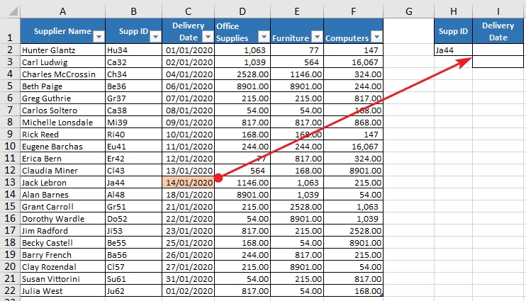
VLOOKUP returns a wrong date if you forget to specify the Match mode (range_lookup) but XLOOKUP returns the correct date. See image below

XLOOKUP easily returns Multiple Columns

XLOOKUP belongs to the new Dynamic array formulas in excel that allows one to return multiple results to a range of cells.

This range is commonly known as Spill Range which can either be multiple rows/columns or a table.

Using the previous data, let us look up the delivery date, Office supplies, Furniture, and Computers for Supplier Id “Ja44”?

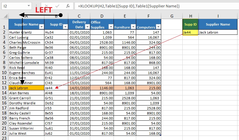
XLOOKUP easily Looks to the Left

Another beauty of XLOOKUP is its ability to do a left lookup without the help of another function. (Neither INDEX nor VLOOKUP can do this dynamically without the help of the MATCH Function)

For VLOOKUP to look up to the left you have to modify it as shown below

=VLOOKUP(H2,IF({1,0},Table1[Order ID],Table1[Product ID]),2,FALSE)

XLOOKUP does NOT break up with the Insertion/Deletion of Columns/rows

Unlike VLOOKUP, XLOOKUP handles Insertions and Deletion of rows/columns smoothly just like INDEX & MATCH

But unlike INDEX & MATCH, this is not a combo formula but a simple and easy to understand the single function

VLOOKUP can handle the insertion & deletion of columns with the help of the MATCH function

XLOOKUP easily looks Vertically and Horizontally

No more need for HLOOKUP or the Combo formula INDEX & MATCH, XLOOKUP takes the day.

XLOOKUP easily does a WILD CARD search

XLOOKUP has the ability to do a search using a fuzzy or approximate Match. This is where the text values are not an exact match.

No need to install Fuzzy Lookup Add-In for Excel!

XLOOKUP Calculates Faster than INDEX/MATCH

Excel MVP Wyn Hopkins has done a good speed test. See for yourself

XLOOKUP returns a cell reference

Just like INDIRECT, INDEX, or OFFSET, XLOOKUP returns a  reference to a cell and thus can be used to create dynamic ranges.

XLOOKUP easily looks up bottom-up and Up-bottom

You can easily search for the last or first entry in a list using XLOOKUP.

XLOOKUP easily returns a Value if no match is found

Prior to XLOOKUP, one has to nest a look-up function inside IFERROR.

This is no longer the case!

XLOOKUP has an inbuilt “if no match” found which can return a value or nest another function.

XLOOKUP 2-way lookup

INDEX and MATCH have been a favorite of many while doing a 2-way lookup but XLOOKUP may change the hearts of many.

This requires a nested XLOOKUP. The trick is to spill the return array first and then use another XLOOKUP to search for it

XLOOKUP returns non-adjacent columns

It is easy for XLOOKUP to return data from multiple adjacent columns.

You just select them in the return arrays and the values will be spilled.

For non-adjacent columns, you need to nest the IF function to select the columns.

=XLOOKUP(
   H2,
    Sales[Supp ID],
      IF({1,0},Sales[Delivery Date],Sales[Computers])
        )

NB: IF function can only help you return 2 non-adjacent columns.

When you want more than 2 columns then use SWITCH or CHOOSE functions

=XLOOKUP(H2,Sales[Supp ID],
SWITCH({1,2,3},1,Sales[Delivery Date],2,Sales[Computers],Sales[Supplier Name]))

or CHOOSE Function

=XLOOKUP(H2,Sales[Supp ID],
CHOOSE({1,2,3},Sales[Delivery Date],Sales[Computers],Sales[Supplier Name]))

Bonus: If you wish to return All returned values in one cell, wrap the XLOOKUP with TEXTJOIN

=TEXTJOIN(",",TRUE,
XLOOKUP(H2,Sales[Supp ID],CHOOSE({1,2,3},Sales[Delivery Date],Sales[Computers],Sales[Supplier Name]))
)

Conclusion:

XLOOKUP may not be the panacea for all excel lookup problems, nor may it be the “Excel Chicken Soup of the Soul” but if you are looking for an all-in-one lookup function…then this is it.

Sadly this function is only available in Office365. If you don’t have Office365, then learn, VLOOKUP, HLOOKUP, INDEX & MATCH, & LOOKUP.

Now you know WTF…What’s The Fuss is all about!

Download Worksheet