Having done a series on Verticle lookup, it is only fair to touch on the Horizontal lookup.

HLOOKUP function is the most popular function for this kind of lookup but it has a number of limitations and thus one may need to know a few other ways you can carry out a Horizontal lookup.

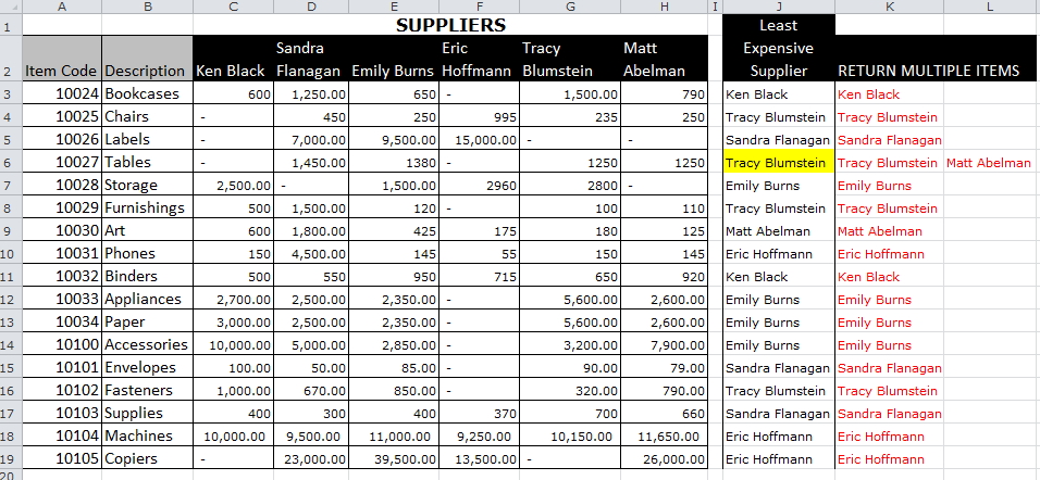
For example, given below data of suppliers, items supplied and prices for each supplier, Can you extract the least expensive supplier(s)?

Most users would jump to HLOOKUP for this task. but it is the least effective based on its limitations. I will start with the most effective–VBA

VBA

We are going to use a  simple code I learned from the Videos I recommended in the REVERSE LOOKUP USING VBA article.

It  just requires a little tweaking and it will be able to do a horizontal lookup and return duplicates

Function HL(Price As Range, LookupPrices As Range, k As Integer)

CustomerNames = LookupPrices.Rows(1).Row - k

HL = ""

For Each cell In LookupPrices
If cell.Value = Application.WorksheetFunction.Min(Price.Value) Then

HL = HL & Cells(CustomerNames, cell.Column).Value & " ; "

End If
Next cell
End Function

Results

Here is the Breakdown:

►Create a Function that accepts 3 parameters

Function HL(Price As Range, LookupPrices As Range, k As Integer)

1.  What to lookup (Price As Range)
2. Where to Lookup (LookupPrices As Range)
3.  Offset factor from Customer names row (k)

►Declare what you want to return:

• Customer Names which are  k row(s) above the Lookup Prices

CustomerNames = LookupPrices.Rows(1).Row - k

NB: You have to create a helper column to store this k Factor which is calculated by a simple formula (=ROW()-ROW($I$2))

►Declare a variable that will hold your results.

HL = ""

NB. The variable should be in the same Name as your Function

►Declare a variable that the function will loop through

For Each cell In LookupPrices
If cell.Value = Application.WorksheetFunction.Min(Price.Value)

For every cell that contains the Minimum Price in the Range return the customer name & separate the result(s) with ( ; )

NB: Learn more about Calling Worksheet Functions In VBA

HL = HL & Cells(CustomerNames, cell.Column).Value & " ; "

DOWNLOAD WORKSHEET 

INDEX & MATCH

Other than VBA, I would highly recommend using a combination of INDEX & MATCH. Apply below formula per every item

=INDEX($C$2:$H$2, MATCH(MIN(C3:H3),C3:H3,0))

How It Works;

►MIN(C3: H3) Returns the minimum price for the item in row 3

MIN(C3:H3)=600

►MATCH(MIN(C3: H3), C3: H3,0) Returns the relative position of the price given the range C3:H3

MATCH(600,C3:H3,0)=1

►INDEX($C$2:$H$2, 1) returns the customer name given the column number by MATCH

NB: This formula does not return multiple duplicates as shown below in the case of Tables. There are 2 suppliers with the same minimum price yet it only returns the first one “Tracy Blumstein”

How do we return multiple items in a Horizontal Lookup?

You need to use a combination of INDEX, SMALL &  IF array formula.

{=IFERROR(
  INDEX($C$2:$H$2,0,
     SMALL(
      IF(
       $C3:$H3=MIN($C3:$H3),COLUMN($C3:$H3)-COLUMN($C3)+1)
     ,COLUMN(A$1))),""
)}

NB: To understand the array formula, see the explanation on this article  OR watch this Video

DOWNLOAD WORKSHEET 

HLOOKUP

This is my least recommended formula because of its Limitations, the biggest being Look up value must be in the top row of a table.

=HLOOKUP(MIN(C3:H3),C3:$H$20,ROW($C$20:$H$20)-(ROW(A3)-ROW($A$1)),FALSE)

How It Works;

►MIN(C3:H3) Returns the minimum price for the item in row 3

MIN(C3:H3)=600

►C3:$H$20 Returns a dynamic table_array that ensures that prices per item are at the top row.

►ROW($C$20:$H$20)-(ROW(A3)-ROW($A$1)) Ensures the added customers names row at the end of the table is returned

NB: This formula does not return Multiple items,  So it is wrong in the case of “Tables” above

No idea how to make HLOOKUP return multiple rows. If you know, Please share in the comments below.

DOWNLOAD WORKSHEET