Array formulas come in handy when you want to look up and sum a large amount of data. Array formulas can replace multiple normal formulas, perform multiple calculations and return a single value as a result.

For example, using below Main sales data in Quantity and a lookup price table, Calculate total sales for customer Brosina Hoffman?

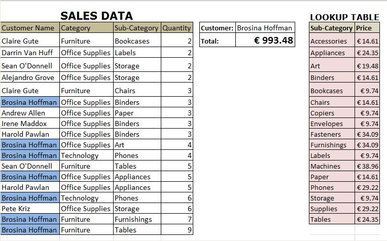
There are 3 ways to do this;

1.Using a combination of SUM, SUMIF & IF 

{=SUM(
   SUMIF(LookupProducts,SalesProduct,Price)*
     IF(Customers=G4,1,0)*
       QuantitySold
)}=993.48

How this works;

►SUMIF(LookupProducts, SalesProduct, Price) is used to fetch the price per product

{9.74;9.74;9.74;9.74;14.61;14.61;14.61;14.61;
14.61;19.48;29.22;24.35;24.35;24.35;29.22;9.74;
34.09;24.35}

►IF(Customers=G4,1,0) compares the customer name in the customers’ list and returns an array of 1 & 0

{0;0;0;0;0;1;0;0;0;1;1;0;1;0;1;0;1;1}

►QuantitySold  returns an array of all quantity  of sold

{2;2;2;2;3;3;3;3;3;4;4;5;5;5;6;6;7;9}

Since this is an array formula the SUM function sums the products of all arrays and it iterates the process described above for each value.

2. Using a combination of  SUM, IF & TRANSPOSE

{=SUM(
  (QuantitySold)*
     IF(SalesProducts=TRANSPOSE(LookupProducts),TRANSPOSE(Price),0)*(Customer=G4))}=993.48

This formula works almost the same as one above the only difference being IF & TRANSPOSE  are used to fetch the Prices;

►IF(SalesProducts=TRANSPOSE(LookupProducts), TRANSPOSE(Price)) is used to creates an array of prices per product.

{0,0,0,0,9.74,0,0,0,0,0,0,0,0,0,0,0,0;0,0,0,0,0,0,0,0,0,0,
9.74,0,0,0,0,0,0;0,0,0,0,0,0,0,0,0,0,0,0,0,0,9.74,0,0;0,0,
0,0,0,0,0,0,0,0,0,0,0,0,9.74,0,0;0,0,0,0,0,14.61,0,0,0,0,0,
0,0,0,0,0,0;0,0,0,14.61,0,0,0,0,0,0,0,0,0,0,0,0,0;0,0,0,0,0,
0,0,0,0,0,0,0,14.61,0,0,0,0;0,0,0,14.61,0,0,0,0,0,0,0,0,0,0,0,
0,0;0,0,0,14.61,0,0,0,0,0,0,0,0,0,0,0,0,0;0,0,19.48,0,0,0,0,0,0,
0,0,0,0,0,0,0,0;0,0,0,0,0,0,0,0,0,0,0,0,0,29.22,0,0,0;0,0,0,0,0,0,
0,0,0,0,0,0,0,0,0,0,24.35;0,24.35,0,0,0,0,0,0,0,0,0,0,0,0,0,0,0;0,
24.35,0,0,0,0,0,0,0,0,0,0,0,0,0,0,0;0,0,0,0,0,0,0,0,0,0,0,0,0,29.22,
0,0,0;0,0,0,0,0,0,0,0,0,0,0,0,0,0,9.74,0,0;0,0,0,0,0,0,0,0,0,34.09,0,
0,0,0,0,0,0;0,0,0,0,0,0,0,0,0,0,0,0,0,0,0,0,24.35}

Everything else is the same.

NB: TRANSPOSE function is used to make the vertical lookup table to be horizontal. As a result, we can multiply the vertical array (the Main table) and the horizontal array (the lookup table) to create a 2-dimensional array formula.

3.  Using a combination of SUM & LOOKUP

{=SUM(
   LOOKUP(SalesProducts,LookupProducts,Price)*
     QuantitySold*
      (Customer=G4))}=993.48

Again this is the same as the first formula the ONLY difference is we use LOOKUP instead of SUMIF to fetch Prices

►LOOKUP(SalesProducts,LookupProducts, Price) is used to creates an array of prices per product.

{9.74;9.74;9.74;9.74;14.61;14.61;14.61;14.61;
14.61;19.48;29.22;24.35;24.35;24.35;29.22;9.74;
34.09;24.35}

NB:

• These are array formulas so remember to Ctrl + Shift +Enter
• For LOOKUP to work you have to sort the data in lookup table ascendingly

Download Worksheet for Practice.

Would You Like To Receive Such an Article in Your Email?

Join our mailing list to receive our weekly Articles!

No Huff! No Fluff! No Spam!

SUBSCRIBE!

You have Successfully Subscribed!