In our everyday life as Human Resources professionals, we encounter large volumes of data that would normally require us to extract some information from.

This article highlights some of the basic excel functions that are aimed at making this process simpler and exciting!

Some of the basic functions we shall look into are:

• SUM
• SUMIFS
• DATEDIF
• TODAY
• COUNT
• COUNTIF(S)
• COUNTBLANK
• COUNTA
• MAX
• MIN
• UPPER
• LOWER
• PROPER
• TRIM
• CONCATENATE/ CONCAT
• VLOOKUP
• XLOOKUP
• INDEX AND MATCH

NOTE: The range of data in the excel worksheet used in the illustrations below has been converted to a table.

Discover more on Excel Tables and how you can incorporate them in your data analysis.

EXCEL SUM & SUMIFS FUNCTION

SUM is a basic excel formula that allows you to add up numbers in a range of cells.

For example, using the below data, what is the total salary for the whole company?

=SUM(F3:F23)=$3,049,059

SUM function can be taken a notch higher if you want to sum data based on criteria.

Using the example above, how do you calculate salary per department? In this scenario, we use SUMIFS Function

=SUMIFS(sum_range, criteria_range, criteria)

SUMIFS adds the cells in a range (sum_range) based on cells in a criteria range and criteria. NB: the length of the sum_range must be equal to the length of the criteria range

Read more on the SUMIF function.

=SUMIFS(Employees[Salary],Employees[Department],H5) = 573,459 this is the total salary for all staff working in HR

WORKING WITH DATES IN EXCEL

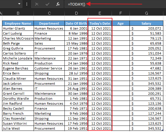
TODAY

Often in HR, we need to calculate variables like the age or the length of service for staff in reference to today’s date.

Using the TODAY function you will always have accurate variables as the function recalculates itself and always returns the current day’s date(ps. This was done on 12 Oct 2021).

Read more on the TODAY function of excel.

DATEDIF

DATEDIF calculates the number of days, months, or years between two dates.

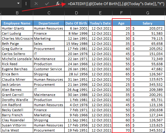
For instance, to get the age given their date of birth and today’s date, the DATEDIF function will come in handy.

The syntax for this formula can be stated in the following variations:

=DATEDIF(Start date, End date, "Y") – This will return the number of complete years between two dates, such as when calculating the age of an individual.

=DATEDIF(Start date, End date, "M") – This will return the number of complete months between two dates.

=DATEDIF(Start date, End date, "D") – This will return the number of days between two dates.

So, given a set of data with the employee’s dates of birth, we can calculate their age in years as shown below.

Read more on Date and Time Functions.

EXCEL COUNT FUNCTIONS

COUNT

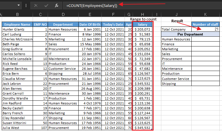
COUNT returns a count of numbers values ONLY.

Numbers can be negative/positive, percentages, dates, times, fractions, and formulas that return numbers. 

Empty cells and text values are ignored. For these, we use COUNTBLANK and COUNTA respectively

When you have a set of data as shown below and would like to know how many employees have a salary figure, the COUNT formula would be the easiest way to get the figure.

COUNTIF

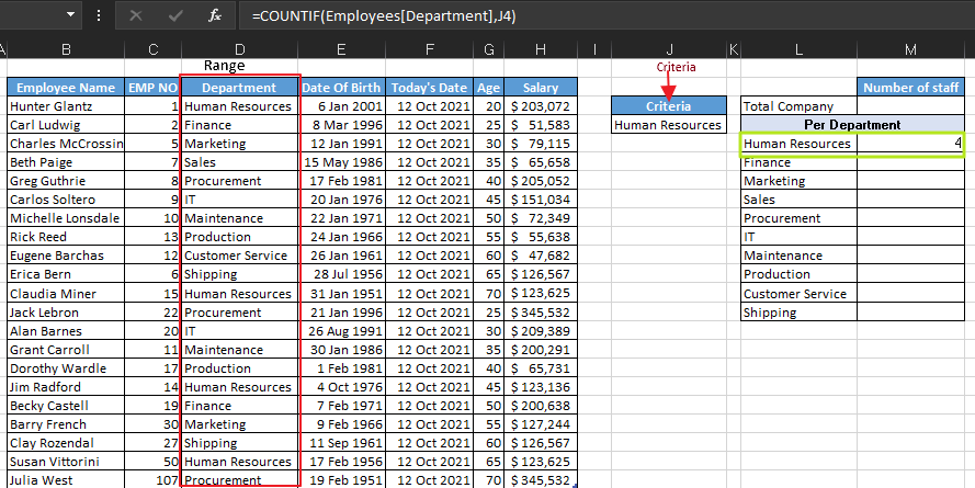
COUNTIF is used to count the number of cells that meet a given criterion; for example, to count the number of staff in a particular department in a staff list.

Basically, it can be elaborated as;

=COUNTIF(Where are the data you are counting?, What are you looking for?)

=COUNTIF(Range, Criteria)

COUNTIFS

This function returns the number of cells that meet more than one criterion. In the example below, we have used the COUNTIF formula to return all staff in the Human Resources department whose age is above 30.

=COUNTIFS(Criteria_Range1, Criteria1,Criteria_Range2,Criteria2...)

Read more on the COUNTIFS formula.

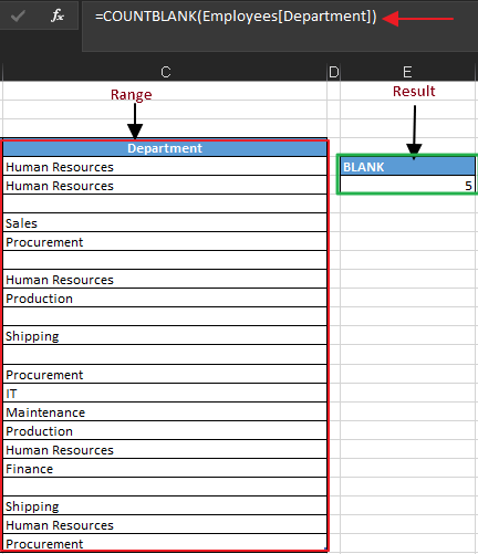
COUNTBLANK

This function returns a count of empty cells in a range. Cells that contain text, numbers, errors, spaces, etc. are not counted.

=COUNTBLANK(range)

In the example below, we can know the number of blank cells in the “Department” column in the table.

COUNTA

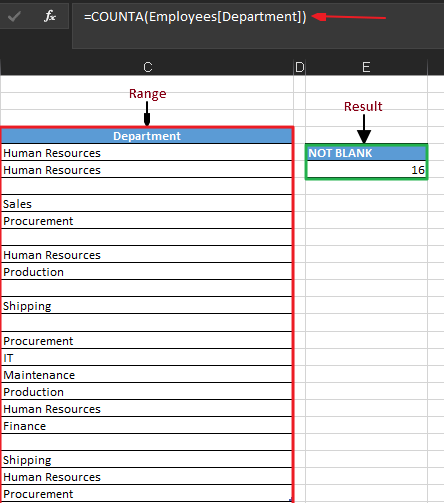
This function returns the count of cells that contain numbers, text, logical values, error values, and empty text (” “).

This function does not count empty cells.

=COUNTA(Range)

In the example below, we can know the number of cells in the “Department” row that are not blank.

EXCEL MAX AND MIN FUNCTIONS

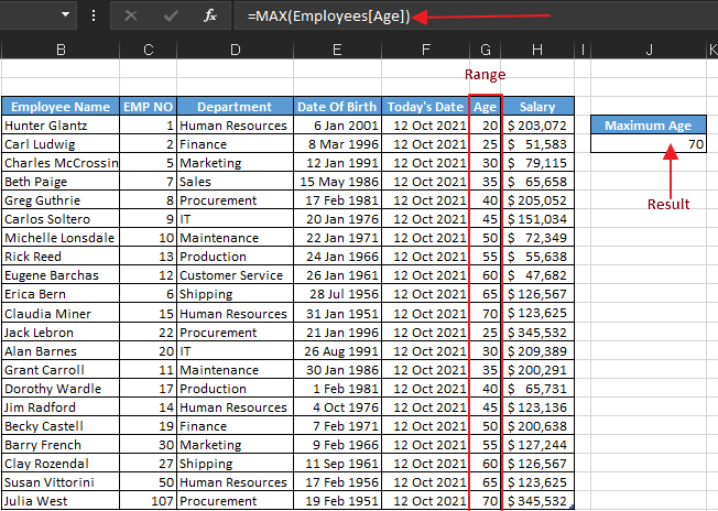
MAX

MAX returns the largest value in a range or set of values.

In the example below, the MAX formula is used to return the age of the oldest staff.

Read more on the MAX function.

MIN

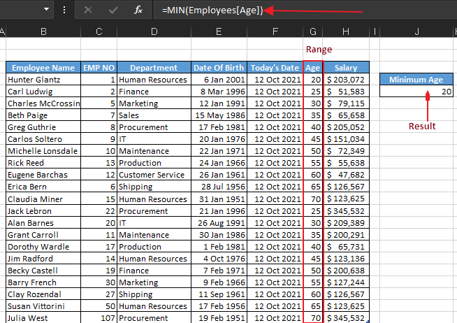
MIN returns the smallest value in a range or set of values.

In the example below, the MAX formula is used to return the age of the youngest staff

Read more on the MIN function.

EXCEL UPPER, LOWER, PROPER & TRIM FUNCTIONS

UPPER

This converts all lowercase characters in a text string to uppercase.

=UPPER(text)

Explore more on how to use the UPPER function.

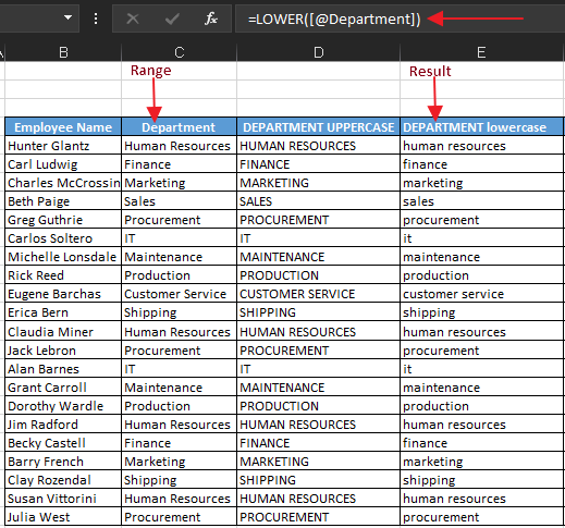
LOWER

This function converts all uppercase characters in a text string to lowercase.

=LOWER(text)

Explore more on how to use the LOWER function.

PROPER

This function converts the first letters of each word in a string to an Upper case.

It does not affect numbers or punctuations in a given text or string. This function is useful in cleaning up data.

=PROPER(text)

Read more on the PROPER Function of excel.

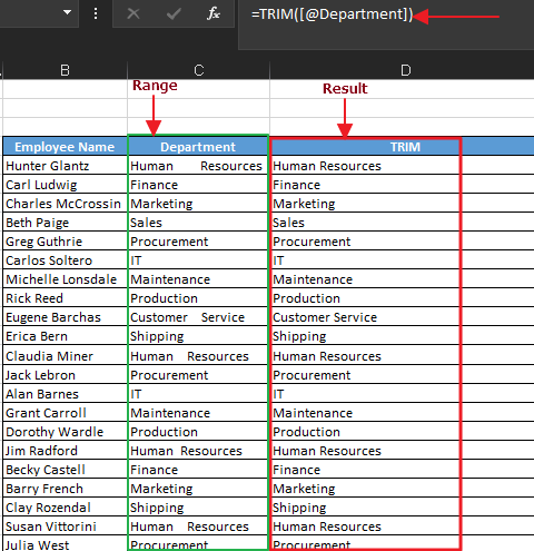
TRIM

This function removes all spaces from text except for single spaces between words.

It is especially useful in cleaning up data.

=TRIM(text)

Explore more on the TRIM function.

EXCEL CONCATENATE/CONCAT FUNCTION

CONCATENATE or CONCAT

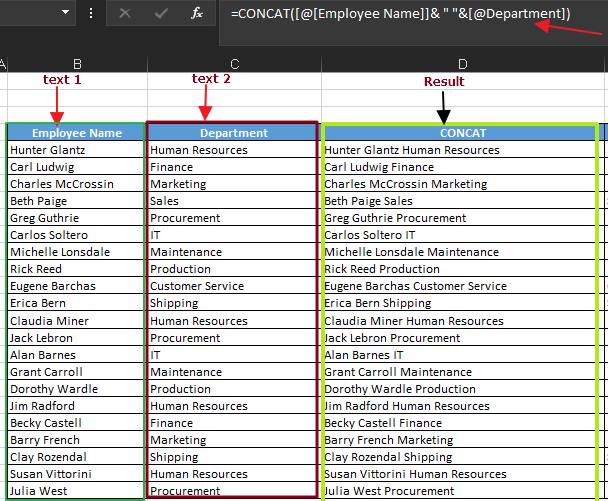
This function allows you to join different texts.

To separate the texts, you need to add space enclosed in double quotation marks as shown in the example below.

Both CONCATENATE and CONCAT have the same logic to generate a result but the CONCAT function only works in excel 2019 and later versions.

=CONCAT(text1,text2.....)

Discover more on the CONCATENATE Function.

EXCEL LOOKUP, INDEX AND MATCH FUNCTIONS

VLOOKUP

VLOOKUP is an excel function that looks up data vertically in a table organized.

VLOOKUP only looks up to the left of the lookup value but you can modify this for it to look up to the right

Note: Lookup values MUST appear in the first column of the table to be passed to VLOOKUP.

=VLOOKUP(lookup_value, table array, col_index_num, range_lookup)

In the illustration below, we want to look up the department that particular employee comes from using the VLookup function.

XLOOKUP

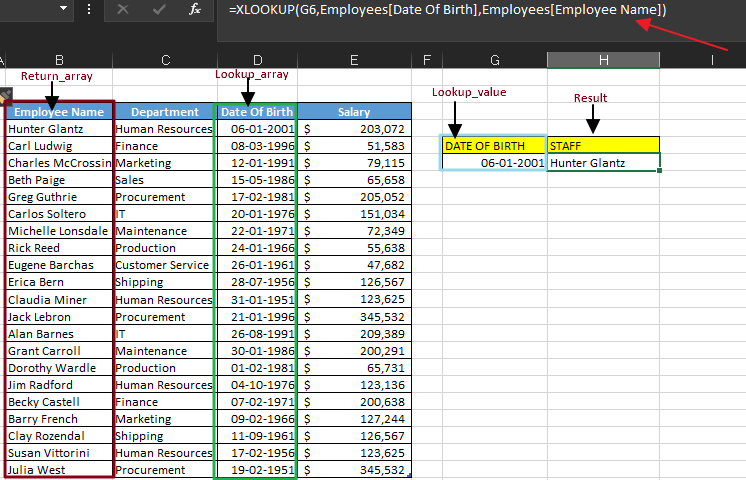
This function is a modern and flexible replacement for older functions like VLOOKUP, HLOOKUP, and LOOKUP.

XLOOKUP looks up both to the left and right and also both vertically or horizontally

ranges.

=XLOOKUP(lookup_value, lookup_array, return_array...)

Explore more on the XLOOKUP function of excel

Note: this function is only available in Excel 365 version

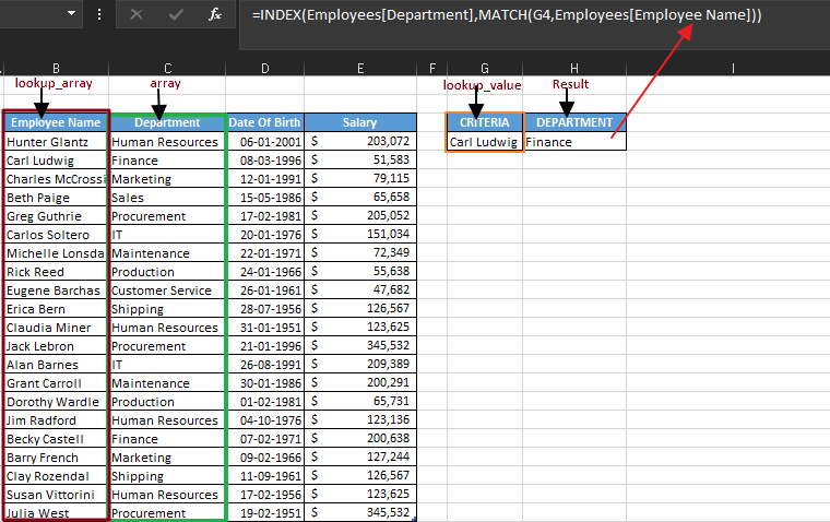
INDEX MATCH FORMULA

This formula is the combination of two functions INDEX and MATCH.

INDEX returns the value of a cell in a table based on the column and row number.

MATCH returns the position of a cell in a row or column.

= INDEX (array, MATCH(lookup_value, lookup_array, 0))

Explore more on the Index Match formula in excel and the various ways it can be used.

In the set of data below, if we have a list of staff and we want to know which department they are in, we can use the INDEX MATCH formula as shown.

CONCLUSION

With the large amount of data encountered in HR, utilizing excel functions and features makes it easier to retrieve and analyze data.

Data analytics enables us to get insight from the data that we have and come up with useful information such as the rate of attrition, the return on investment on our employees, the cost of recruitment et cetera.