

Sequential numbers can be used as unique identifiers and an easy way to maintain a count. Below is how to highlight non-sequential numbers in excel.
Steps:
- Select the area to apply Conditional formatting
- Go to Conditional formatting → New rule ► Use a Formula to determine cells to format
- Use this formula =RIGHT(B3,3)+0<>RIGHT(B2,3)+1
- RIGHT(B3, 3) extracts the last three characters in a string e.g. 001 (this is a Text-Number and not a number)
- Any math operation will convert a text number to a real number. This is why we add zero =RIGHT(B3,3)+0
- <>RIGHT(B2,3)+1 check if the current number is equal to the previous number plus 1
- Apply the formatting on all the cells whose result will be TRUE
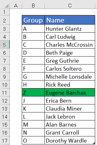
How to Highlight non-alphabetical series
=CHAR(65) to CHAR(90) result in A to Z in excel
So following the above steps use this formula =CHAR(ROW(A65))<>$B3
NB: ROW(A65) results to 65 and the number will be incremental as you scroll down

Recent Comments